3. Model Data
3.1. Stellar Grid Models
The stellar grids are the backbone (or another important structural body-part analogy) of Twinkle and essential to any SED modeling effort. These are stellar atmopsheric models of flux from the star at a range of wavelengths that have been calculated/generated for a stars at a range of temperatures, solar-relative metallicities, and surface gravities. Click here for more information.
These models of wavelength vs. flux are what Twinkle uses to determine the best fit to the input photometric band data and calulate stellar parameters for the observe information.
Twinkle relies on two main atmospheric models: The Kurucz Atlas 9 (Kurucz 1993) and the NextGen atmospheric models (Hauschildt et al. 1999).
Both model files need to be in the project path as shown in the Directory Structure section of the Set-Up Page and listed in the JSON input file ['folders']['topdir']/['folders']['supportdir']/StellarGridModels/ (e.g., twinkle-master/Inputs_and_Models/StellarGridModels/).
For quick access you can find the models on the Github page here.
Note
I have primarily set ATLAS9 for SED modeling late B-spectral type stars, while the NextGen models are best for A-K spectral types.
Note
You can set the model you want to use in the user input file under the model column, and this can be changed for different stars in your input file.
3.2. ATLAS9
A description of the ATLAS9 models can be found in this file README. It includes a description of model temperature ranges, wavelength ranges, and grid steps. There’s also a table of which models are optimal for a given spectral type.
Note
There are also newer (I think) ATLAS9 models that can be accessed here.
Right now, the code only has access to ATLAS9 grid models with stellar metallicities relative to solar of 0.0 and -0.5. To include more metallicities, feel free to download more metallicity folders from the author, and add it to the ATLAS9 directory labeled as k[x][s], where x is either m for minus (-) or p for positive (+), and s refers to the two digit absolute solar relative metallicity value (Z = [M/H]).
The file format of the ATLAS9 models are in standard FITS format. Each file corresponds to flux for a star at a given metallicty and temperature.
For instance, km05_10000.fits is the FITS file for the ATLAS9 atmospheric stellar model at 10000K for metallicity of Z=-0.5.
Each file has a Primary header, and a second Binary Table that has 12 columns, the first corresponding to the wavelength, and the next 11 corresponding to the surface flux units ( \(\mathrm{ergs}\ \mathrm{cm}^{-2}\ \mathrm{s}^{-1} \mathrm{Å}^{-1}\)) at different surface gravities (\(10\log(g)\); from 0 to 50.0 in increments of 0.5).
from astropy.io import fits
import numpy as np

hdu = fits.open('km05_10000.fits')
hdu.info()

>> Filename: km05_10000.fits
>> No.    Name      Ver    Type      Cards   Dimensions   Format
    0  PRIMARY       1 PrimaryHDU      27   ()
    1                1 BinTableHDU     56   1221R x 12C   [1E, 1E, 1E, 1E, 1E, 1E, 1E, 1E, 1E, 1E, 1E, 1E]

temp = hdu[0].header['TEFF']
data = hdu[1].data
colnames = np.array(hdu[1].columns.names)

print(temp)
>> 10000

print(colnames)
>> array(['WAVELENGTH', 'g00', 'g05', 'g10', 'g15', 'g20', 'g25',
'g30','g35', 'g40', 'g45', 'g50'], dtype='<U10')
We can see the Binary Table is a 1221 row by 12 column table, where the values in the row for the WAVELENGTH column is the wavelength of the flux, and the values in all the other columns are the flux at a given wavelength for the surface gravity listed in the column name (g00, g05, etc.)
3.3. NextGen
As I mentioned before, you should specify to the code to use the NextGen atmospheric grid models for spectral types A-K. I originally downloaded the spectra (.spec) files from the late Dr. France Allard’s page.
The most readily accessible models the code can use are of solar metalicity (Z=0), with corresponding surface gravities of log(g) from 3.5 to 5.5 in increments of 0.5.
The current processed files are in the NextGen folder with each file labeled in the format of lteNextGen_[TEMP]_[GRAV]_[MET].txt. TEMP is the stellar temperature, GRAV is the surface gravity, and MET is the metallicity. Each file is a two-column text file, where the first column is wavelength in Angstroms, and the second is flux in \(\mathrm{ergs}\ \mathrm{cm}^{-2}\ \mathrm{s}^{-1} \mathrm{Å}^{-1}\).
Each of these files is created using the (XXX module - treat_NextGenSpecModels) function, which loads the raw spec files, and outputs the lte format text files. The spec files are provided, so feel free to extract more spec files for your use. These currently include Z=-0.5, 0, 0.5,. If you want more, either download them yourself, or contact me.
3.4. Photometric Filter Response Curves
The relative spectral response (RSR) curve files contain information on how a given photometric filter response is distributed across a wide-band spectrum. Basically, each filter or instrument that observes a star has a varying weighted response to the light across a wide-band wavelength regime.
For instance, the Ks-band in the NIRC2 instrument on Keck looks like this:
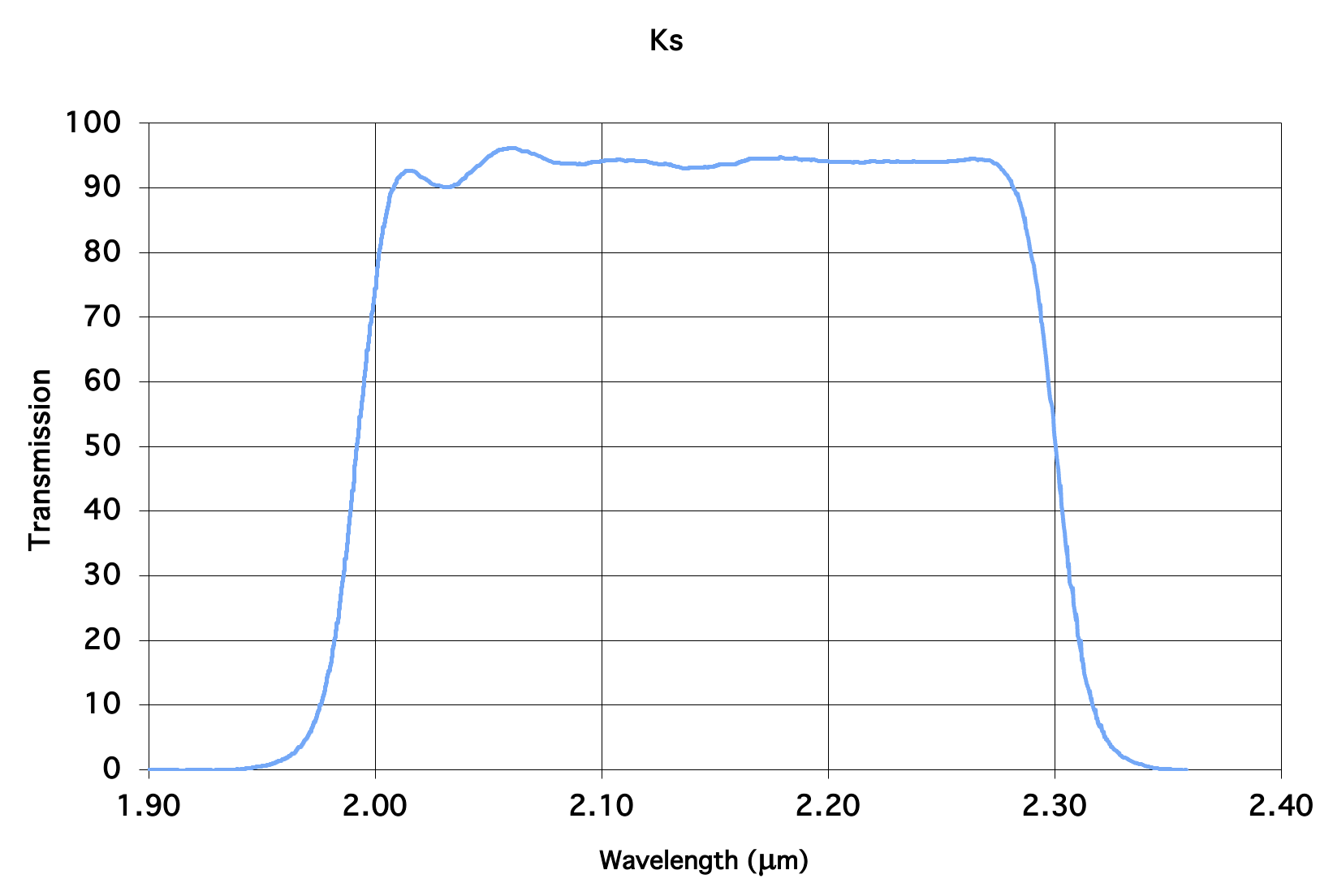
The image shows the percentage of light that passes through the filter at a given wavelength in the range of 1.9 to 2.4 microns. Twinkle takes this filter (and other relevant ones) and convolves it with the modeled photospheric emission and sums the flux over that bandpass. We then use the summed flux at the central or isophotal wavelength for the flux at that wavelength.
All the filter files should be placed in the project path as shown in the Directory Structure of the Set-Up page and listed in the JSON input file ['folders']['topdir']/['folders']['supportdir']/RSR/ (e.g., twinkle-master/Inputs_and_Models/RSR/).
A list of available filters can be found in the Filters ReadME Text file in the downloaded project folders or download it here. The readme file also has references of where the filters were obtained, as well as information on what the header line for each filter file contains.
Important
All the relative spectral responses are exactly that. All the \(\lambda\mathrm{RSR}\) needs to be divided out
Note
The list of available filters may not be up to date in the readme file, so take a look in the RSR folder to see for sure.
Note
The filters available at the moment are from WISE, NIRC2, Spitzer MIPS, 2MASS, Johnson, Bessel, Tycho, Hipparcos, IRAS, Herschel/PACS, Akari, MSX, DENIS, and early Gaia G
If you want to create your own reponse curve to be read by Twinkle, it needs to be in the format like the example below:
#!33526.0[0,f]/ 8.1787e-12[1,f]/ 1.2118e-13[2,f]/ 8.8560e13[3,f]/ 3.0954e-21[4,f]/ 5.81111186e-23[5,f]/
wav     trans
2.53	2.26020E-06
2.54	1.49067E-07
2.55	8.14902E-08
2.56	8.88398E-08
2.57	2.95261E-06
2.58	2.07337E-06
2.59	1.35089E-06
2.60	9.12231E-07
2.61	1.37115E-04
2.62	4.50420E-04
2.63	3.53399E-04
2.64	2.84451E-04
2.65	3.09208E-04
2.66	3.31515E-04
2.67	3.93895E-04
2.68	1.26369E-04
2.69	1.92212E-04
2.70	3.03133E-04
2.71	3.22107E-03
2.72	2.84188E-03
2.73	1.68663E-03
2.74	1.25387E-03
2.75	2.69065E-03
2.76	4.98080E-03
2.77	8.50181E-03
2.78	1.62622E-02
2.79	3.18548E-02
2.80	5.55571E-02
2.81	8.18826E-02
2.82	1.00599E-01
2.83	1.08435E-01
2.84	1.07130E-01
2.85	1.03211E-01
2.86	9.86364E-02
2.87	9.34111E-02
2.88	8.85451E-02
2.89	8.78927E-02
2.90	9.18103E-02
2.91	9.93230E-02
2.92	1.07880E-01
2.93	1.15297E-01
2.94	1.21435E-01
2.95	1.26631E-01
2.96	1.31301E-01
2.97	1.36525E-01
2.98	1.41426E-01
2.99	1.44692E-01
3.00	1.45670E-01
3.01	1.46651E-01
3.02	1.47629E-01
3.03	1.46977E-01
3.04	1.44036E-01
3.05	1.40446E-01
3.06	1.35546E-01
3.07	1.30319E-01
3.08	1.24114E-01
3.09	1.18887E-01
3.10	1.15948E-01
3.11	1.18235E-01
3.12	1.26728E-01
3.13	1.39792E-01
3.14	1.51876E-01
3.15	1.61022E-01
3.16	1.67228E-01
3.17	1.71801E-01
3.18	1.75720E-01
3.19	1.79313E-01
3.20	1.82250E-01
3.21	1.83885E-01
3.22	1.85519E-01
3.23	1.86498E-01
3.24	1.87151E-01
3.25	1.85517E-01
3.26	1.83558E-01
3.27	1.82251E-01
3.28	1.82905E-01
3.29	1.87802E-01
3.30	1.97930E-01
3.31	2.11320E-01
3.32	2.25364E-01
3.33	2.37775E-01
3.34	2.46269E-01
3.35	2.50809E-01
3.36	2.50155E-01
3.37	2.45255E-01
3.38	2.39704E-01
3.39	2.33204E-01
3.40	2.26344E-01
3.41	2.22425E-01
3.42	2.26673E-01
3.43	2.39408E-01
3.44	2.56686E-01
3.45	2.72365E-01
3.46	2.82162E-01
3.47	2.86735E-01
3.48	2.87356E-01
3.49	2.86049E-01
3.50	2.85069E-01
3.51	2.84123E-01
3.52	2.83142E-01
3.53	2.82195E-01
3.54	2.79257E-01
3.55	2.74685E-01
3.56	2.68803E-01
3.57	2.62272E-01
3.58	2.55740E-01
3.59	2.51493E-01
3.60	2.50186E-01
3.61	2.53127E-01
3.62	2.58680E-01
3.63	2.63906E-01
3.64	2.66519E-01
3.65	2.67173E-01
3.66	2.66519E-01
3.67	2.65864E-01
3.68	2.64886E-01
3.69	2.63905E-01
3.70	2.62959E-01
3.71	2.62631E-01
3.72	2.61978E-01
3.73	2.59365E-01
3.74	2.51201E-01
3.75	2.35883E-01
3.76	2.12399E-01
3.77	1.81141E-01
3.78	1.44984E-01
3.79	1.07456E-01
3.80	7.41737E-02
3.81	4.86325E-02
3.82	3.02827E-02
3.83	1.84864E-02
3.84	1.13661E-02
3.85	7.16909E-03
3.86	4.55959E-03
3.87	2.84651E-03
3.88	1.74250E-03
3.89	1.23167E-03
3.90	1.02164E-03
3.91	8.02813E-04
3.92	6.07500E-04
3.93	5.73868E-04
3.94	4.59873E-04
3.95	3.82785E-04
3.96	2.86414E-04
3.97	1.65103E-04
3.98	8.90678E-05
3.99	1.07293E-05
4.00	2.50800E-05
4.01	1.09646E-05
4.02	7.26393E-06
4.03	3.35434E-06
4.04	1.85713E-06
4.05	1.25583E-06
4.06	3.07414E-06
4.07	2.88010E-07
4.08	2.04559E-06
4.09	1.87641E-06
4.10	3.59610E-07
4.11	8.21776E-07
4.12	2.07859E-07
4.13	1.65235E-07
4.14	8.78261E-07
4.15	7.21157E-06
4.16	1.27185E-05
4.17	1.52398E-05
4.18	1.19801E-05
4.19	8.77279E-06
4.20	8.39405E-08
4.21	7.66556E-08
4.22	6.82299E-08
4.23	5.86596E-08
4.24	4.86981E-08
4.25	3.61247E-07
4.26	2.98404E-08
4.27	2.37471E-07
4.28	1.58801E-07
4.29	1.23527E-07
4.30	7.62651E-09
4.31	5.16056E-09
4.32	3.44259E-09
4.33	5.00370E-08
4.34	1.46749E-09
4.35	9.29218E-10
4.36	5.96720E-10
4.37	9.27918E-09
4.38	2.61393E-10
4.39	1.92866E-10
4.40	1.42893E-10
4.41	3.01995E-09
4.42	8.15566E-11
4.43	5.96411E-11
4.44	4.39302E-11
4.45	4.59865E-10
4.46	4.38655E-10
4.47	1.65626E-11
4.48	1.10462E-11
4.49	8.69131E-12
4.50	5.77133E-12
4.51	3.29224E-12
4.52	9.82124E-11
4.53	1.84342E-12
4.54	1.56024E-12
4.55	9.84088E-13
4.56	4.17741E-08
4.57	3.22998E-08
4.58	9.32817E-08
4.59	4.49760E-08
4.60	3.64174E-08
4.61	3.22430E-08
4.62	1.07881E-07
4.63	3.55356E-08
4.64	1.11800E-07
4.65	5.14086E-08
4.66	6.36910E-08
4.67	1.25550E-07
4.68	3.30855E-08
4.69	5.71578E-08
4.70	1.31398E-07
4.71	3.67771E-10
4.72	5.15403E-10
4.73	3.58288E-10
4.74	1.22023E-10
4.75	1.43187E-09
4.76	8.20126E-10
4.77	2.43753E-10
4.78	4.45502E-11
4.79	1.23754E-10
4.80	1.59258E-09
4.81	3.92911E-11
4.82	4.67054E-11
4.83	3.01035E-13
4.84	1.47793E-11
4.85	3.59938E-10
4.86	1.11179E-09
4.87	2.88131E-10
4.88	3.14406E-12
4.89	3.95215E-10
4.90	9.30857E-10
4.91	1.02656E-13
4.92	3.40000E-11
4.93	8.20791E-10
4.94	1.40053E-09
4.95	6.06202E-10
4.96	3.05907E-09
4.97	3.26378E-09
4.98	2.89679E-09
4.99	7.16273E-09
5.00	1.34892E-08
5.01	9.80818E-09
5.02	7.69841E-09
5.03	6.08489E-09
5.04	5.25853E-09
5.05	5.46752E-09
5.06	5.52964E-09
5.07	5.71913E-09
5.08	5.91831E-09
5.09	5.95088E-09
5.10	5.66020E-09
5.11	5.81703E-09
5.12	5.67324E-09
5.13	5.87914E-09
5.14	5.89222E-09
5.15	5.68971E-09
5.16	5.47403E-09
5.17	5.36634E-09
5.18	5.28784E-09
5.19	5.23565E-09
5.20	5.20635E-09
5.21	5.05278E-09
5.22	5.29119E-09
5.23	5.40880E-09
5.24	5.37939E-09
5.25	5.83981E-09
5.26	6.32319E-09
5.27	6.62049E-09
5.28	6.78712E-09
5.29	7.20189E-09
5.30	7.41094E-09
5.31	7.77345E-09
5.32	8.49192E-09
5.33	8.62589E-09
5.34	7.87790E-09
5.35	8.21757E-09
5.36	8.62257E-09
5.37	8.37114E-09
5.38	8.09033E-09
5.39	8.49852E-09
5.40	8.51481E-09
5.41	8.45287E-09
5.42	8.42989E-09
5.43	8.38103E-09
5.44	6.81654E-09
5.45	7.78330E-09
5.46	8.45604E-09
5.47	8.33528E-09
5.48	8.07391E-09
5.49	8.44299E-09
5.50	8.08382E-09
5.51	7.72123E-09
5.52	7.40761E-09
5.53	7.00922E-09
5.54	6.56823E-09
5.55	6.29712E-09
5.56	5.80072E-09
5.57	5.19318E-09
5.58	4.89928E-09
5.59	4.44848E-09
5.60	4.01411E-09
5.61	3.66471E-09
5.62	3.48826E-09
5.63	3.04512E-09
5.64	2.87518E-09
5.65	2.44212E-09
5.66	2.30813E-09
5.67	2.04815E-09
5.68	1.57789E-09
5.69	1.38779E-09
5.70	1.10526E-09
5.71	8.49860E-10
5.72	8.93287E-10
5.73	8.29930E-10
5.74	9.19094E-10
5.75	1.01381E-09
5.76	1.20128E-09
5.77	1.43123E-09
5.78	1.58279E-09
5.79	1.69088E-09
5.80	1.87931E-09
5.81	2.04234E-09
5.82	2.39313E-09
5.83	2.44889E-09
5.84	2.69332E-09
5.85	2.96957E-09
5.86	3.11075E-09
5.87	3.24685E-09
5.88	3.62211E-09
5.89	3.82139E-09
5.90	3.84102E-09
5.91	3.98799E-09
5.92	4.12517E-09
5.93	4.59882E-09
5.94	4.49428E-09
5.95	4.71630E-09
5.96	4.77517E-09
5.97	5.11156E-09
5.98	5.05920E-09
5.99	5.10501E-09
6.00	5.39567E-09
6.01	5.18985E-09
6.02	5.21279E-09
6.03	5.17678E-09
6.04	5.08212E-09
6.05	5.33041E-09
6.06	4.82739E-09
6.07	4.75222E-09
6.08	4.73914E-09
6.09	4.69343E-09
6.10	4.80459E-09
6.11	4.74566E-09
6.12	4.79477E-09
6.13	4.98418E-09
6.14	5.43485E-09
6.15	5.85951E-09
6.16	6.77403E-09
6.17	6.59433E-09
6.18	6.82945E-09
6.19	7.80614E-09
6.20	7.63629E-09
6.21	1.06346E-08
6.22	1.16863E-08
6.23	1.34305E-08
6.24	1.89279E-08
6.25	2.57856E-08
6.26	3.52412E-08
6.27	4.52360E-08
6.28	5.67006E-08
6.29	6.62703E-08
6.30	7.19540E-08
6.31	3.54057E-08
6.32	1.02459E-07
6.33	9.63523E-08
6.34	8.45931E-08
6.35	7.88126E-08
6.36	8.21431E-09
6.37	6.65636E-09
6.38	1.09384E-08
6.39	6.11095E-08
6.40	5.49047E-08
6.41	1.09056E-07
6.42	1.04844E-07
6.43	7.46967E-08
6.44	9.62857E-08
6.45	9.41302E-08
6.46	7.31950E-08
6.47	8.99505E-08
6.48	3.24136E-08
6.49	8.93297E-08
6.50	7.76031E-08
The file snippet shows the response curve data for the Wide-Field Infrared Survey Explorer (WISE) W1 filter. The second line contains the column header for the wavelength (microns) and the transmission.
The first line contains a header with bandpass specific information in the following format:
#!N0[0,f]/ N1[1,f]/ N2[2,f]/ N3[3,f]/ N4[4,f]/ N5[5,f]/
where
N0 = Isophotal wavelength (Angstroms)
N1 = Vega zero point flux (\(\mathrm{ergs}\ \mathrm{cm}^{-2}\ \mathrm{s}^{-1} \mathrm{Å}^{-1}\))
N2 = uncertainty in Vega zero point flux (\(\mathrm{ergs}\ \mathrm{cm}^{-2}\ \mathrm{s}^{-1} \mathrm{Å}^{-1}\))
N3 = Isophotal frequency (Hz)
N4 = Vega zero point flux (\(\mathrm{ergs}\ \mathrm{cm}^{-2}\ \mathrm{s}^{-1} \mathrm{Å}^{-1}\))
N5 = uncertainty in Vega zero point flux (\(\mathrm{ergs}\ \mathrm{cm}^{-2}\ \mathrm{s}^{-1} \mathrm{Å}^{-1}\))
All this information can be found in the readme file linked above.